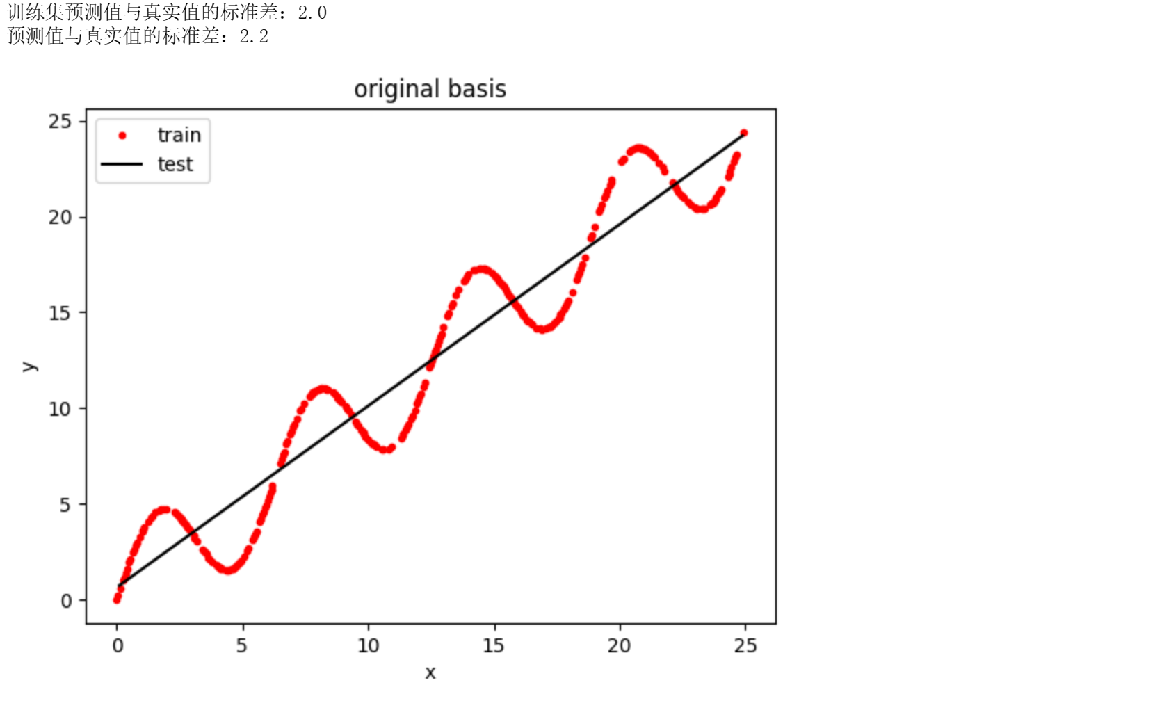
nndl编程练习2:线性模型练习题解

本文最后更新于:几秒前

说明

请按照填空顺序编号分别完成 参数优化,不同基函数的实现

1
2
3
4
5
6
7
8
9
10
11
import numpy as np
import matplotlib.pyplot as plt

def load_data(filename):
"""载入数据。"""
xys = []
with open(filename, 'r') as f:
for line in f:
xys.append(map(float, line.strip().split()))
xs, ys = zip(*xys)
return np.asarray(xs), np.asarray(ys)

不同的基函数 (basis function)的实现

填空顺序 2

请分别在这里实现“多项式基函数”以及“高斯基函数”

其中以及训练集的x的范围在0-25之间

1
2
3
4
5
6
7
8
9
10
11
12
13
14
15
16
17
18
19
20
21
22
23
24
25
26
27
28
29
def identity_basis(x):
ret = np.expand_dims(x, axis=1)
return ret
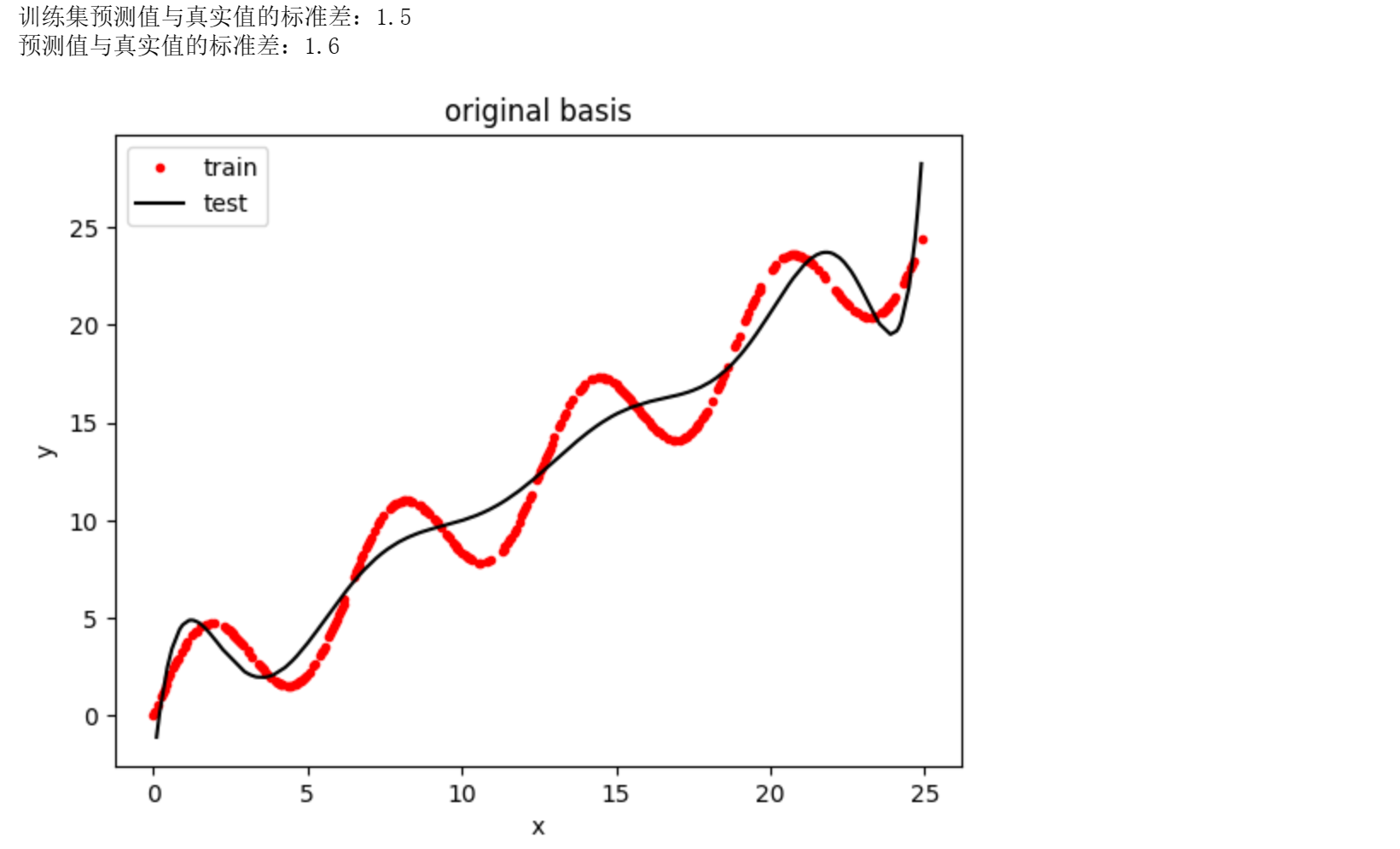
def multinomial_basis(x, feature_num=10):
x = np.expand_dims(x, axis=1) # shape(N, 1)
ret = [x]
# 分别乘幂
for i in range(2,feature_num+1):
ret.append(x**i)
#将乘幂的结果连起来
ret=np.concatenate(ret,axis=1)
print(ret.shape)
return ret
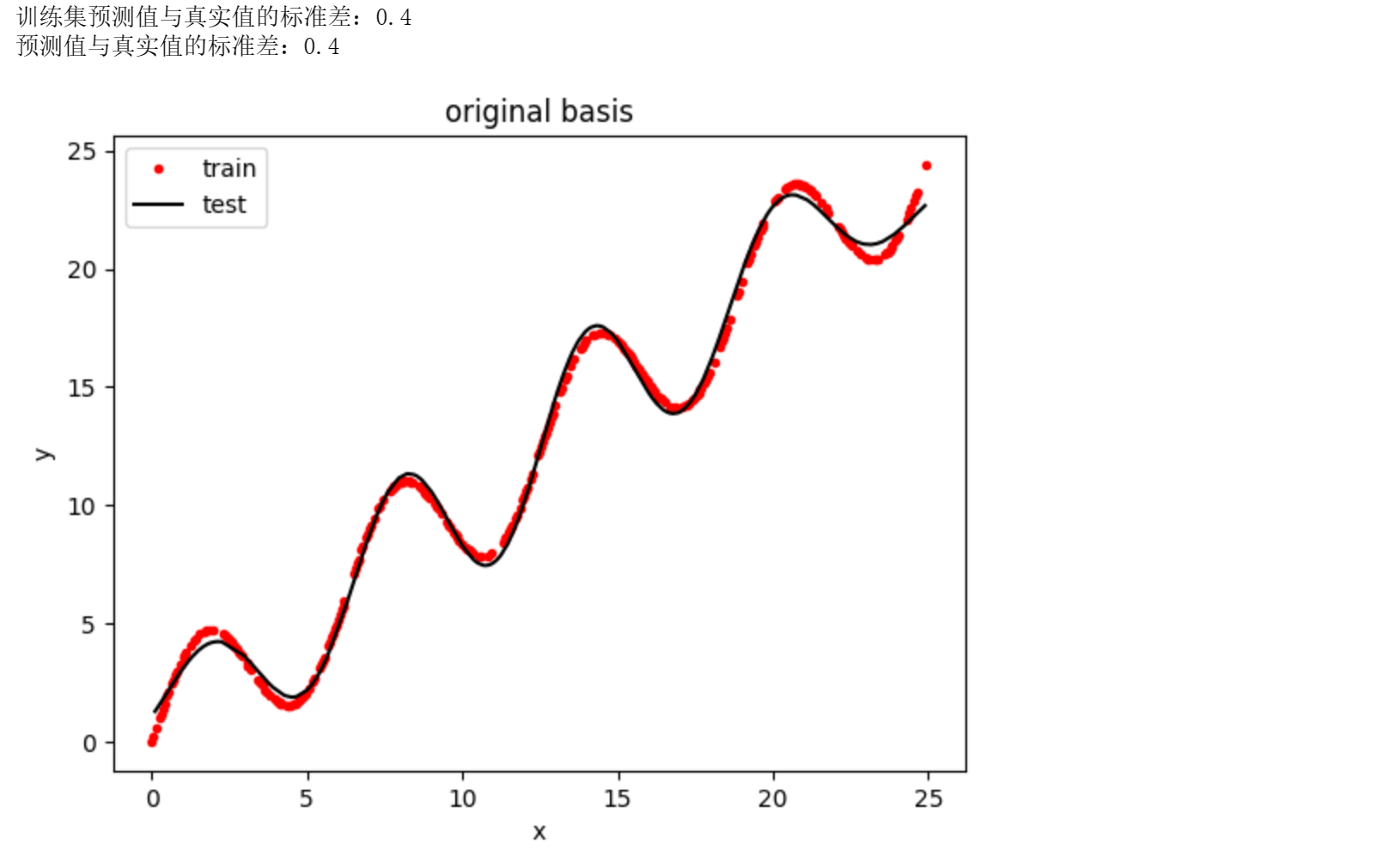

def gaussian_basis(x, feature_num=10):
'''高斯基函数'''
#==========
#todo '''请实现高斯基函数'''
#==========
# 高斯基函数
centers = np.linspace(0,25,feature_num)
s = centers[1]-centers[0]
phi = np.expand_dims(x,axis=1)
x = np.concatenate([phi]*feature_num,axis=1)
t =( x - centers)/s
ret = np.exp(- 0.5 * t ** 2)
return ret

多项式基函数:
$$
\phi_j(x) = x^j
$$
高斯基函数:
$$
\phi_j(x) = \exp\lbrace -{ {(x-\mu_j)^2} \over {2s^2} } \rbrace = \exp \lbrace - {1\over 2} ({ (x-\mu_j)\over s}) ^2 \rbrace
$$

返回一个训练好的模型

填空顺序 1 用最小二乘法进行模型优化

填空顺序 3 用梯度下降进行模型优化

先完成最小二乘法的优化 (参考书中第二章 2.3中的公式)

再完成梯度下降的优化 (参考书中第二章 2.3中的公式)

在main中利用训练集训练好模型的参数,并且返回一个训练好的模型。

计算出一个优化后的w,请分别使用最小二乘法以及梯度下降两种办法优化w

1
2
3
4
5
6
7
8
9
10
11
12
13
14
15
16
17
18
19
20
21
22
23
24
25
26
27
28
29
30
31
32
33
34
35
36
37
38
39
40
def main(x_train, y_train,):
"""
训练模型,并返回从x到y的映射。

"""
#加入1序列,作为训练时的常量$b$

#在这里更换基函数
basis_func = multinomial_basis
phi0 = np.expand_dims(np.ones_like(x_train), axis=1)
phi1 = basis_func(x_train)
phi = np.concatenate([phi0, phi1], axis=1)


#==========
#todo '''计算出一个优化后的w,请分别使用最小二乘法以及梯度下降两种办法优化w'''
#==========
#最小二乘法,其中np.linalg.pinv()求的是phi的伪逆矩阵
w = np.dot(np.linalg.pinv(phi),y_train)
#梯度下降
#损失函数
# def dj(theta,phi,y):
# return phi.T.dot(np.dot(phi,theta)-y) * 2.0 / len(phi)

# def gradient(phi,y,initial_theta, eta=0.001, n_iters=10000):
# w = initial_theta
# for i in range(n_iters):
# w = w - eta * dj(w,phi,y)
# return w
# initial_theta = np.zeros(phi.shape[1])
# w = gradient(phi,y_train,initial_theta)

def f(x):
phi0 = np.expand_dims(np.ones_like(x), axis=1)
phi1 = basis_func(x)
phi = np.concatenate([phi0, phi1], axis=1)
y = np.dot(phi, w)
return y

return f

最小二乘法训练模型是直接计算解
$$
\pmb w^* = (\pmb {XX}^\top)^{-1} \pmb X\pmb y
$$
其中,$(\pmb {XX}^\top)^{-1} \pmb X$被称为$\pmb X^\top$的伪逆矩阵,因为$\pmb X^{-1}$不是满秩的,所以需要用伪逆矩阵表示,伪逆矩阵可以用np.linalg.pinv()计算。

梯度下降分为两步,其一是计算梯度,其二是梯度下降

首先,梯度计算式可以表示为
$$
\begin{align}
{\partial \mathcal L} \over {\partial w} & = { {\partial {1\over n} \sum_{n=1}^n (wx^{(i)}+b-y^{(i)})}^2 \over {\partial w} } \\
& = {1\over n} \sum_{n=1}^n { {\partial (wx^{(i)}+b-y^{(i)})}^2 \over {\partial w} } \\
& = {1\over n}\sum_{n=1}^n \ 2 · (wx^{(i)}+b-y^{(i)}) · { {\partial (wx^{(i)}+b-y^{(i)})} \over {\partial w} } \\
& = {2\over n}\sum_{n=1}^n \ (wx^{(i)}+b-y^{(i)}) ·x^{(i)}
\end{align}
$$
最后的式子可以转写为矩阵表达式
$$
{ {\partial \mathcal L} \over {\partial \pmb w} } = {2\over n} ·\pmb x^\top (\pmb w\pmb x-\pmb y)
$$
然后,梯度下降表达式为
$$
\pmb w = \pmb w-\eta { \partial L \over {\partial \pmb w} }
$$
权重的初始值可以全部赋0,这样就完成了梯度下降的搭建。

评估结果

没有需要填写的代码,但是建议读懂

1
2
3
4
5
6
7
8
9
10
11
12
13
14
15
16
17
18
19
20
21
22
23
24
25
26
27
28
29
30
31
32
33
34
35
36
37
38
39
40
def evaluate(ys, ys_pred):
# 计算标准差
"""评估模型。"""
std = np.sqrt(np.mean(np.abs(ys - ys_pred) ** 2))
return std

# 程序主入口(建议不要改动以下函数的接口)
if __name__ == '__main__':
train_file = 'train.txt'
test_file = 'test.txt'
# 载入数据
x_train, y_train = load_data(train_file)
x_test, y_test = load_data(test_file)
print(x_train.shape)
print(x_test.shape)
# 使用线性回归训练模型,返回一个函数f()使得y = f(x)
# 定义训练函数
f = main(x_train, y_train)

y_train_pred = f(x_train)
std = evaluate(y_train, y_train_pred)
print('训练集预测值与真实值的标准差:{:.1f}'.format(std))

# 计算预测的输出值
y_test_pred = f(x_test)
# 使用测试集评估模型
std = evaluate(y_test, y_test_pred)
print('预测值与真实值的标准差:{:.1f}'.format(std))

# 用plt输出图像
#显示结果
plt.plot(x_train, y_train, 'ro', markersize=3)
# plt.plot(x_test, y_test, 'k')
plt.plot(x_test, y_test_pred, 'k')
plt.xlabel('x')
plt.ylabel('y')
plt.title('original basis')
plt.legend(['train', 'test', 'pred'])
plt.show()

结果

原始基函数

image-20230131184451988

多项式基函数

image-20230131184539586

高斯基函数

image-20230131184620340


nndl编程练习2:线性模型练习题解
http://paopao0226.site/post/2477d76.html
作者
Ywj226
发布于
2023年1月31日
更新于
2023年9月23日
许可协议