nndl编程练习3:logistic回归和softmax回归练习题解
本文最后更新于:几秒前
logistic回归
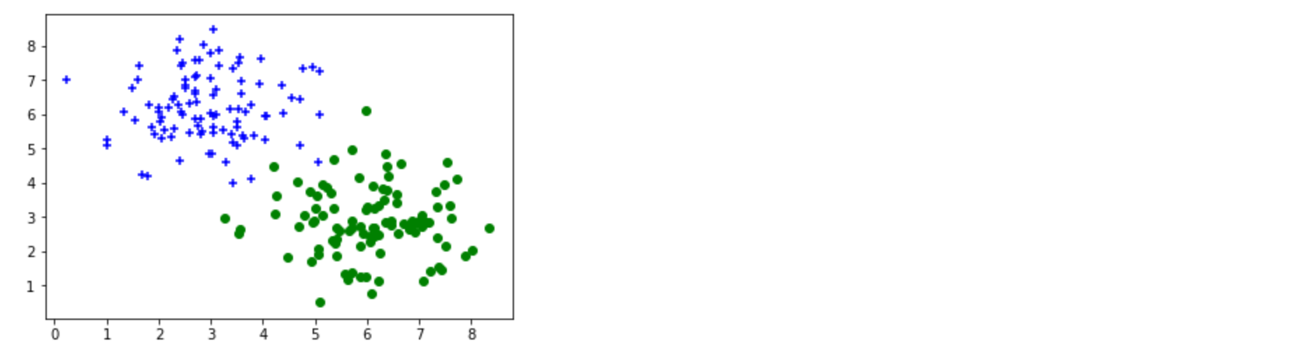
生成数据集, 看明白即可无需填写代码
‘+‘ 从高斯分布采样 (X, Y) ~ N(3, 6, 1, 1, 0).
‘o‘ 从高斯分布采样 (X, Y) ~ N(6, 3, 1, 1, 0)
1 | |
建立模型
建立模型类,定义loss函数,定义一步梯度下降过程函数
填空一:实现sigmoid的交叉熵损失函数(不使用tf内置的loss函数)
logistic线性模型的损失函数为交叉熵损失
$$
\mathcal L(\theta) = -{1\over N}\sum_{n=1}^N (y^{(n)} \log\hat y^{(n)}+(1-y^{(n)})\log (1-\hat y^{(n)}))
$$
在这里解代码在预测值后面加上了一个极小量$\epsilon=10^{-12}$,这个的意义我暂时还不太知晓。
这里的代码做了两个改动,分别对应于两个报错:
TypeError: Input ‘b’ of ‘MatMul’ Op has type float32 that does not match type float64 of argument ‘a’.
解决办法:在报错的行,用tf.cast作强制转型
2
3
4#原代码
#logits = tf.matmul(inp, self.W) + self.b # shape(N, 1)
#修改后代码
logits = tf.matmul(tf.cast(inp,tf.float32), self.W) + self.b # shape(N, 1)TypeError: Expected float32, but got Tensor(“label:0”, shape=(), dtype=float64) of type ‘Tensor’.
解决办法:去掉@tf.function,防止强制转换float为tensor
见代码注释
1 | |
实例化一个模型,进行训练
1 | |
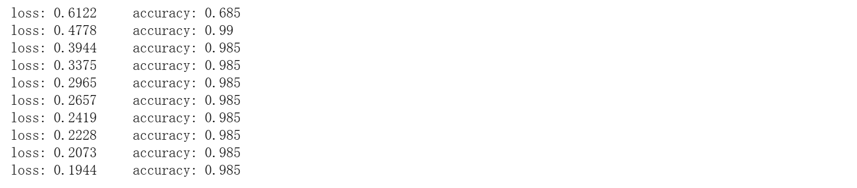
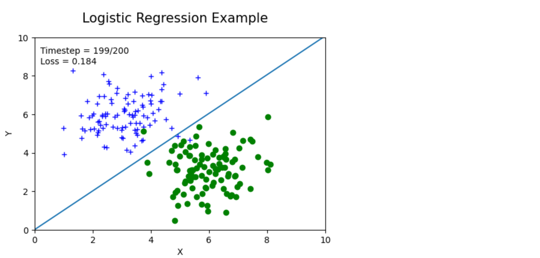
结果展示,无需填写代码
1 | |
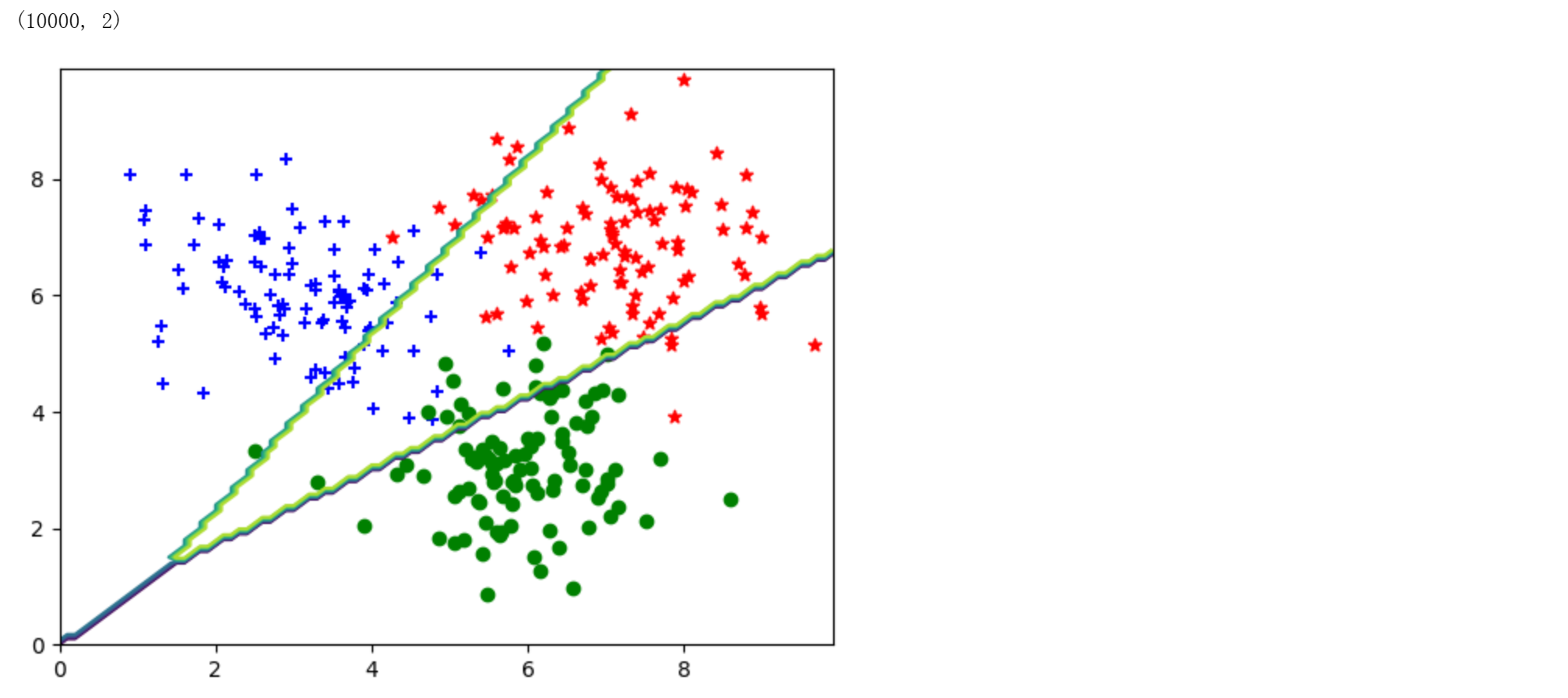
Softmax回归
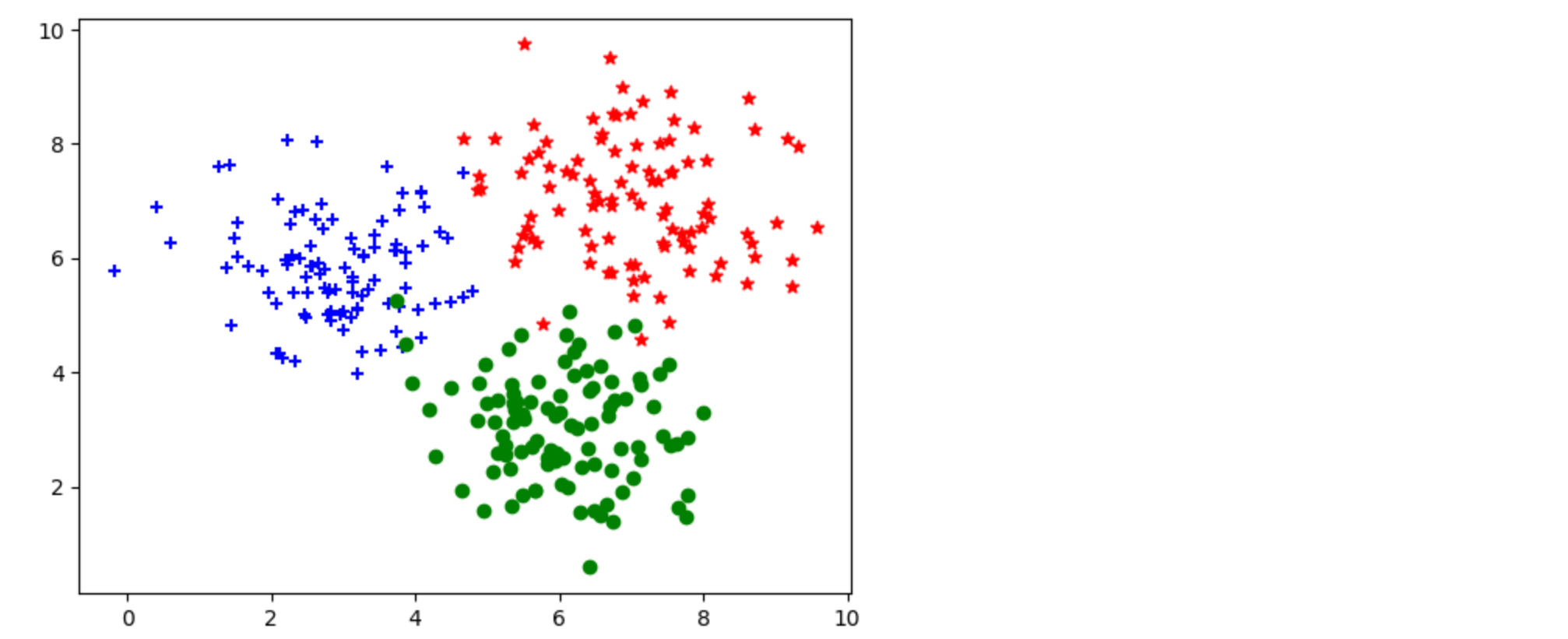
生成数据集, 看明白即可无需填写代码
‘+‘ 从高斯分布采样 (X, Y) ~ N(3, 6, 1, 1, 0).
‘o‘ 从高斯分布采样 (X, Y) ~ N(6, 3, 1, 1, 0)
‘*‘ 从高斯分布采样 (X, Y) ~ N(7, 7, 1, 1, 0)
1 | |
建立模型
建立模型类,定义loss函数,定义一步梯度下降过程函数
填空一:在__init__构造函数中建立模型所需的参数
填空二:实现softmax的交叉熵损失函数(不使用tf内置的loss函数)
1 | |
实例化一个模型,进行训练
1 | |
结果展示,无需填写代码
1 | |
附:对logistic回归的复现
1 | |